
Wave Breaking, roller and undertow
Breaking schemes
There are two breaking algorithms implemented in the model. One takes advantage of the shock–capturing scheme in TVD. It follows the approach of Tonelli and Petti (2009), who successfully used the ability of the nonlinear shallow water equation (NSWE) with a TVD scheme to model moving hydraulic jumps. Thus, the fully nonlinear Boussinesq equations are switched to NSWE at cells where the Froude number exceeds a certain threshold. Following Tonelli and Petti, the ratio of wave height to total water depth is chosen as the criterion to switch from Boussinesq to NSWE, with a threshold value set to 0.8, as suggested by Tonelli and Petti.
The other wave breaking scheme is the original eddy–viscosity scheme used in the previous version of FUNWAVE (Kennedy et al., 2000. To fit the eddy–viscosity method in the TVD scheme, the artificial eddy viscosity terms are:
Note that the form is slightly different from that in Kennedy et al. (2000). The present form was found to give a more stable numerical solution with the cross–derivatives removed. In the present form, \(\nu\) is the artificial eddy viscosity defined by:
where \(\delta_b = 1.2\). In Kennedy et al. (2000), \(B\) varies smoothly from 0 to 1 so as to avoid an impulsive start of breaking and the resulting instability. In the present TVD model, because there is no instability problem found, we adopt a constant value \(B=1\) as breaking is initiated:
The parameter \(\eta_t^*\) determines the onset and cessation of breaking. Following Kennedy et al., a breaking event begins when \(\eta_t\) exceeds some initial threshold value \(\eta_t^{(I)}\), as breaking develops, the wave will continue to break until \(\eta_t\) drops below \(\eta_t^{(F)}\). However, we do not use the smooth transition as in Kennedy et al. because the present TVD scheme did not encounter any instability problem associated with breaking. The values of \(\eta_t^{(I)}\) and \(\eta_t^{(F)}\) can be described by \(C_{brk1} \sqrt{gh}\) and \(C_{brk2} \sqrt{gh}\), respectively, where \(C_{brk1}\) and \(C_{brk2}\) are empirical parameters. In Kennedy et al., \(C_{brk1} = 0.65\) and \(C_{brk2}=0.15\). Choi et al. (2018) showed that \(C_{brk1}\) should be smaller and \(C_{brk2}\) be larger than those in Kennedy et al. to match the laboratory experimental data. For the benchmark test of Vincent and Briggs (1989) for instance, \(C_{brk1} = 0.45\) and \(C_{brk2} = 0.35\) were adopted.
Roller and undertow
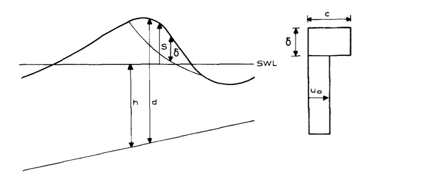
Figure 1. Concept of roller (from Schäffer et al., 1993). Cross-section and assumed velocity profile of a breaking wave with a surface roller.
Roller-induced flux
The general expression of a breaking roller in a Boussinesq-type model was introduced by several authors such as Madsen (1981), Svendsen (1984), and Schäffer et al. (1993). For a one-dimensional case, the roller induced mass flux can be expressed by:
where \(P\) is the total mass flux including the contribution of roller. \(u_0\) is the velocity defined in the figure, \(c\) is the wave celerity, and \(\delta\) is the roller thickness. In FUNWAVE-TVD, we use \(u_\alpha\) to represent the velocity \(u_0\). \(c\) is calculated using:
which is different from Schäffer et al. (1993) who used the local still water depth: \(c=1.3\sqrt{gh}\).
The thickness of roller \(\delta\) can be estimated using the roller geometry shown in Figure 1. However, in the parallelized program, locating the roller region involves cross-core-boundary tracking, that is nontrivial and time-consuming. In FUNWAVE-TVD, we used a rough estimate of the roller thickness based on the correlation between the roller area and the wave height proposed by Svendsen (1984), i.e. :
where \(A\) represents the roller area and \(H\) is the wave height. Based on the roller geometry, the roller area can be estimated as:
where \(L\) is the wave length, \(r\) is a ratio representing the thickness, and \(\delta = rH\). Assuming the wave length can be estimated by \(L = 4 H /\tan \theta\), where \(\tan \theta\) is estimated by \(\tan \theta = \eta_t/c\). According to (9) and (10), the ratio \(r\) can be calculated by:
The ratio \(r\) is limited by the maximum breaking angle (\(20^{\circ}\), Schaffer et al. 1993), resulting in the maxumim value of \(r = 0.1638\).
We further assume the local thickness of the roller at the breaking point is \(\delta = r (\eta^*-\bar{\eta})\), where \(\eta^{*}\) and \(\bar{\eta}\) are the surface elevation at a breaking point and the mean surface elevation, respectively. The final formula for the roller-induced mass flux can be expressed as:
The mean surface elevation is calculated using the time series of surface elevation before the roller estimation.
Roller effect on hydrodynamics
Following Schaffer et al. (1993), the total momentum flux, including the roller contribution, can be expressed as:
The excess momentum effect due to the non-uniform velocity distribution can be calculated using (12) and (13):
or
The roller effect on hydrodynamics can be calculated by adding extra terms, \(R_x\) and \(R_y\), in the momentum equations in the x and y directions, respectively.
The calculation of the undertow uses the local balance of the roller induced momentum flux and the undertow flux. The roller/undertow effect is taken into account in the sediment transport processes.
To set up the roller and its effects, see Physics (dispersion, breaking, friction). An example presenting the roller effect can be found in Sediment Transport in 2D rip channels. To set up output of roller-induced mass flux and undertow flux, see Output.
References
Choi, Y.-K., Shi, F., Malej, M., and Smith, J. M., 2018, “Performance of various shock-capturing-type reconstruction schemes in the Boussinesq wave model, FUNWAVE-TVD”, Ocean Modelling, 131, 86-100. DOI:10.1016/j.ocemod.2018.09.004.
Kennedy, A.B., Chen, Q., Kirby, J.T., Dalrymple, R.A., 2000. “Boussinesq modeling of wave transformation, breaking and runup. I: 1D”. J. Waterway Port Coastal Ocean Eng. 126(1), 39–47.
Madsen, P.A. 1981. “A model for a turbulent bore”. Series paper 28, Inst. Hydrodyn. and Hydraul. Engng, Tech. Univ. Denmark.
Schäffer H. A., Madsen, P.A., Deigaard, R., 1993, A Boussinesq model for waves breaking in shallow water, Coastal Engineering, DOI:10.1016/0378-3839(93)90001-0
Svendsen, LA., Wave Heights and Set-Up in a Surf Zone, 1984, Coastal Engineering, Vol. 8. DOI:10.1016/0378-3839(84)90028-0
Tonelli, M., and M. Petti, 2009. “Hybrid finite volume – finite difference scheme for 2DH improved Boussinesq equations”. Coastal Engineering, 56(5-6), 609-620. DOI:10.1016.j.coastaleng.2009.01.001
Vincent, C.L., Briggs, M.J., 1989. “Refraction-diffraction of irregular waves over a mound”. J. Waterway Port Coastal Ocean Eng. 115 (2), 269–284. DOI:10.1061/(ASCE)0733-950X(1989)115:2(269)