
Ship-wake Module
We have implemented various types of source functions for ship-wave generation.
1) PRESSURE SOURCE TYPE I
Following Ertekin et al. (1986), Wu (1987), and Torsvik et al. (2008), the pressure disturbance with a center point at \((x^*, y^*)\) is given by:
where:
In the rectangle, \(- L/2 \le \tilde{x} - x^*(t) \le L/2\) and \(- W/2 \le \tilde{y} - y^*(t) \le R/2\), and zero outside this region; \(L\) and \(W\) represent the length and width of the pressure source, respectively. \(\alpha_1\), \(\alpha_2\) and \(\beta\) are parameters representing the shape of the draft region, and \(0\le(\alpha_1, \alpha_2, \beta)<1\). They can be evaluated using the block coefficient of a watercraft as described below. (\(\tilde{x}, \tilde{y}\)) is the coordinate system for the pressure disturbance which may be rotated by an angle relative to the Boussinesq coordinate system (\(x,y\)). \(P\) is a parameter controlling the surface displacement. In fact, \(p_a\) is the static depression around the vessel.
In contrast to the formulation of the pressure distribution in the previous study (Torsvik et al., 2008), \(P\) has a unit of meters and can be interpreted as the inverse barometer effect corresponding to the static surface depression for a stationary vessel.
The values of \(\alpha_1\), \(\alpha_2\), and \(\beta\) are shape parameters and can be obtained by adjusting \(\alpha_1\), \(\alpha_1\) and \(\beta\) to get the displaced volume (static submerged volume of the vessel):
which should match a given block coefficient \(C_B\) defined by:
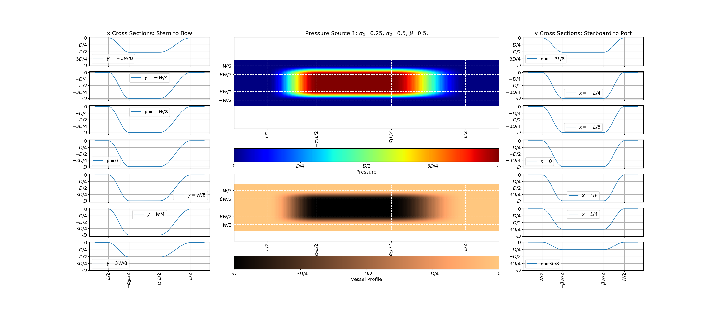
in which \(D\) represents draft of a vessel. An example of how the pressure source is implemented in FUNWAVE is shown in the figure below for \(\alpha_1, \alpha_2,\) and \(\beta = 0.25, 0.5,\) and \(0.5\), respectively. Click on the image to enlarge it.
2) PRESSURE SOURCE TYPE II
Type II of the pressure-type source is formulated following Bayrakter and Beji (2013). David et al. (2017) used this formulation in their tests. The pressure source can be written as:
where \(a\), \(b\) and \(c\) are form parameters. For a slender body, \(a=16.0\), \(b=2.0\) and \(c=16.0\).
3) SLENDER SOURCE TYPE I
For the slender-type source, the additional volume flux induced by ship motion is applied in the mass conservation equation:
where \(dQ\) represents the flux gradient. \(F\) is a parameter which can be determined by the block ratio. The formula is calculated in the rectangle \(- L/2 \le \tilde{x} - x^*(t) \le L/2\) and \(- W/2 \le \tilde{y} - y^*(t) \le R/2\), and zero outside this region.
4) SLENDER SOURCE TYPE II
The Type II of the slender source is similar to the Type I but with two additional parameters representing sizes of bow and stern:
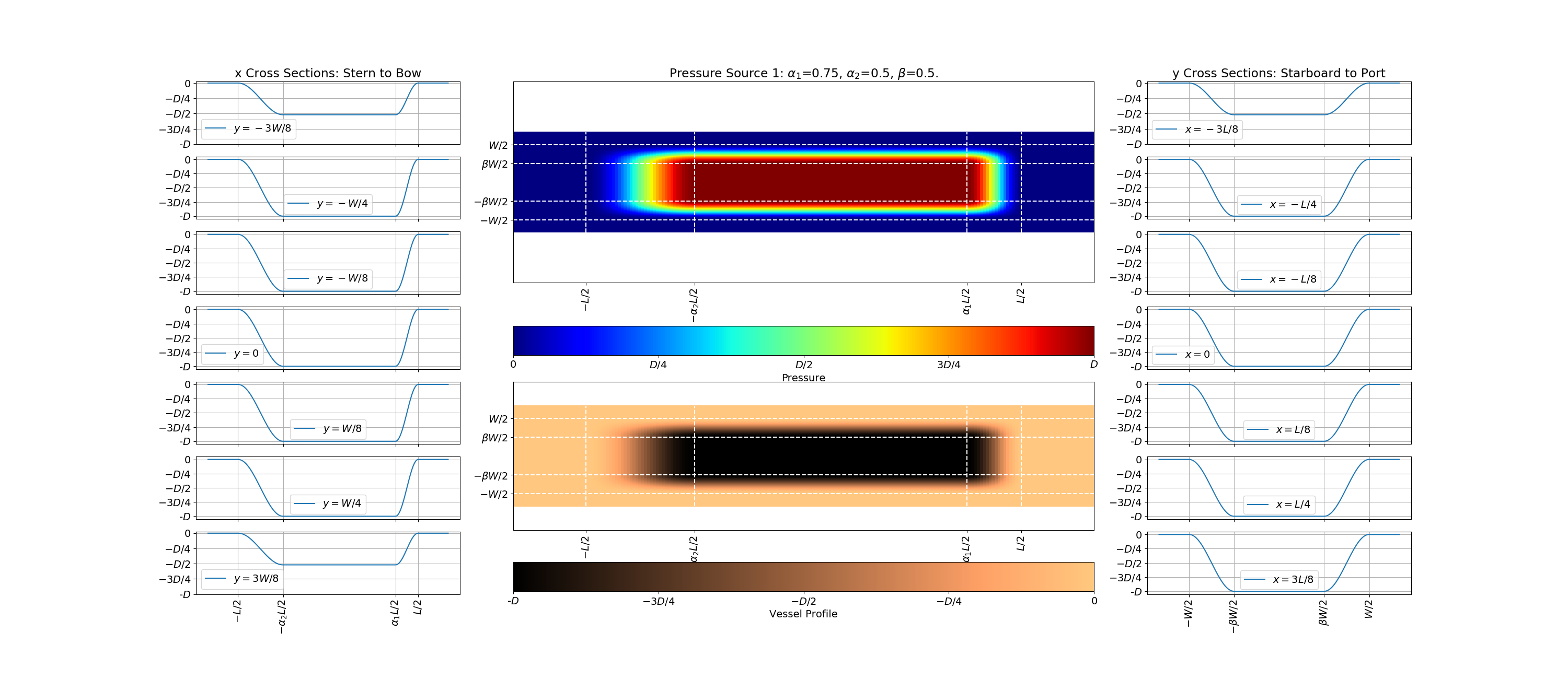
The formula is calculated in the rectangle \(- L/2 \le \tilde{x} - x^*(t) \le L/2\) and \(- W/2 \le \tilde{y} - y^*(t) \le R/2\), and zero outside this region. An example of lengthening the pressure source by increasing \(\alpha_1\) to 0.75.
To set up vessels in the model, see Shipwakes.
References
Bayrakter, D., and S. Beji, (2013). “Numerical simulation of waves generated by a moving pressure field”. Ocean Engineering, 59: 231-239. DOI: 10.1016/j.oceaneng.2012.12.025.
Daved, C.G., V. Roeber, N. Goseberg, and T. Schlurmann, (2017). “Generation and propagation of ship-borne waves - Solutions from a Boussinesq-type model”. Coastal Engineering, 127: 170-187. DOI: 10.1016/j.coastaleng.2017.07.001.
Ertekin, R.C., Webster, W.C., Wehausen, J.V., 1986. “Waves caused by a moving disturbance in a shallow channel of finite width”. Cambridge University Press, 169: 275-292. DOI: 10.1017/S0022112086000630.
Torsvik, T., Pederson, G., Dysthe, K., 2009. “Waves Generated by a Pressure Disturbance Moving in a Channel with Variable Cross-Sectional Topography”. J. of Waterway, Port, Coastal, and Ocean Eng., 135 (3). DOI: 10.1061/(ASCE)0733-950X(2009)135:3(120).
Wu, T.Y., 1987. “Generation of upstream advancing solitons by moving disturbances”. Cambridge University Press, 184: 75-99. DOI: 10.1017/S0022112087002817.