Tide Module

There are two types of boundary conditions developed to incorporate tidal level and/or tidal current into model boundaries. One is an absorbing tidal boundary condition, which is essentially a sponge layer but takes into account a reference value, such as tidal level and tidal current, in the sponge regime. The other a so-called absorbing-generating boundary condition, which treats tidal level and/or tidal current as the background elevation/flow.

Theory

The basic technique follows the sponge layer theory introduced by Larsen and Dancy (1983). Instead of attenuating the surface elevation and flow velocity to zero at the end of a sponge layer, we dampen shortwaves with respect to a reference level based on the method proposed by Chen et al. (1999). The dependent variables (\(\eta, u, v\)) are attenuated as

(112)\[\eta_i = \eta_{ref} + (\eta_i - \eta_{ref})/C_s\]

(113)\[u_i = u_{ref} + (\eta_i - u_{ref})/C_s\]

where \(( )_{ref}\) denotes the reference values which either tidal level or tidal current or both. \(C_s\) is the damping coefficient which is the same as that used in a sponge layer (see sponge layer section for detail), i.e.,

(114)\[C_s = \alpha_s^{\gamma_s^{(i-1)}}\]

in which \(i\) is grid numbers, (\(i = 1, 2, ...\)).

Absorbing tidal boundary condition

For the absorbing tidal boundary condition, the reference values (\(\eta_{ref}, u_{ref}, v_{ref}\)) are tidal levels and tidal current velocities specified either in input.txt or in a separate tide/surge file.

For a constant tidal condition, (\(\eta_{ref}, u_{ref}, v_{ref}\)) are constant, which are specified in input.txt. For example, in the case of tide_abs_1bc_constant in the directory of simple cases,

TIDAL_BC_ABS = T
TideBcType = CONSTANT
TideWest_ETA = 1.0
TideEast_ETA = 1.0

This is a 1D case with a tidal absorbing condition and constant tidal level specified above. The wavemaker can be any types of wavemaker available in the model. In this case, we used WK_REG,

WAVEMAKER = WK_REG
DEP_WK = 8.0
Xc_WK = 150.0
Yc_WK = 0.0
Tperiod = 8.0
AMP_WK = 0.5
Theta_WK = 0.0
Delta_WK = 3.0

The figure shows a snapshot of surface elevation from the model. Note that the irregularity of wave surface is caused by the tidal propagation from both boundaries.

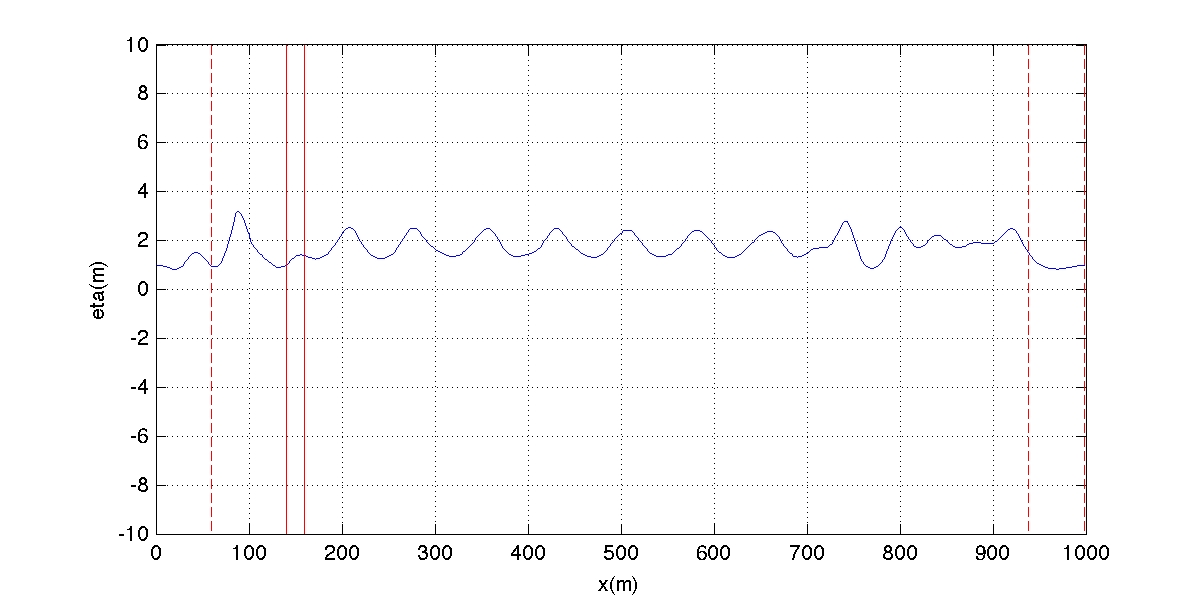
Fig. 1 Output from the case of tidal absorbing boundary condition.

For a time-varying tidal condition, the tidal level and velocity are specified in a file named in input.txt. For example, in the 2D case of tide_abs_2bc_data (same folder), tidal elevations are specified in two files, tide_data_west.txt, tide_data_east.txt, with the parameter TideBcType set as DATA type,

TIDAL_BC_ABS = T
TideBcType = DATA
TideWestFileName = tide_data_west.txt
TideEastFileName = tide_data_east.txt

The format of tidal data follows a list of ‘time, eta, u, v’ as shown in the figure below. In this case, a flat bottom of 8 m is applied in a 2D domain and a regular wavemaker is specified . The following figure demonstrates 2D and 1D section views of surface elevation at different times. Black solid lines denote tidal levels.

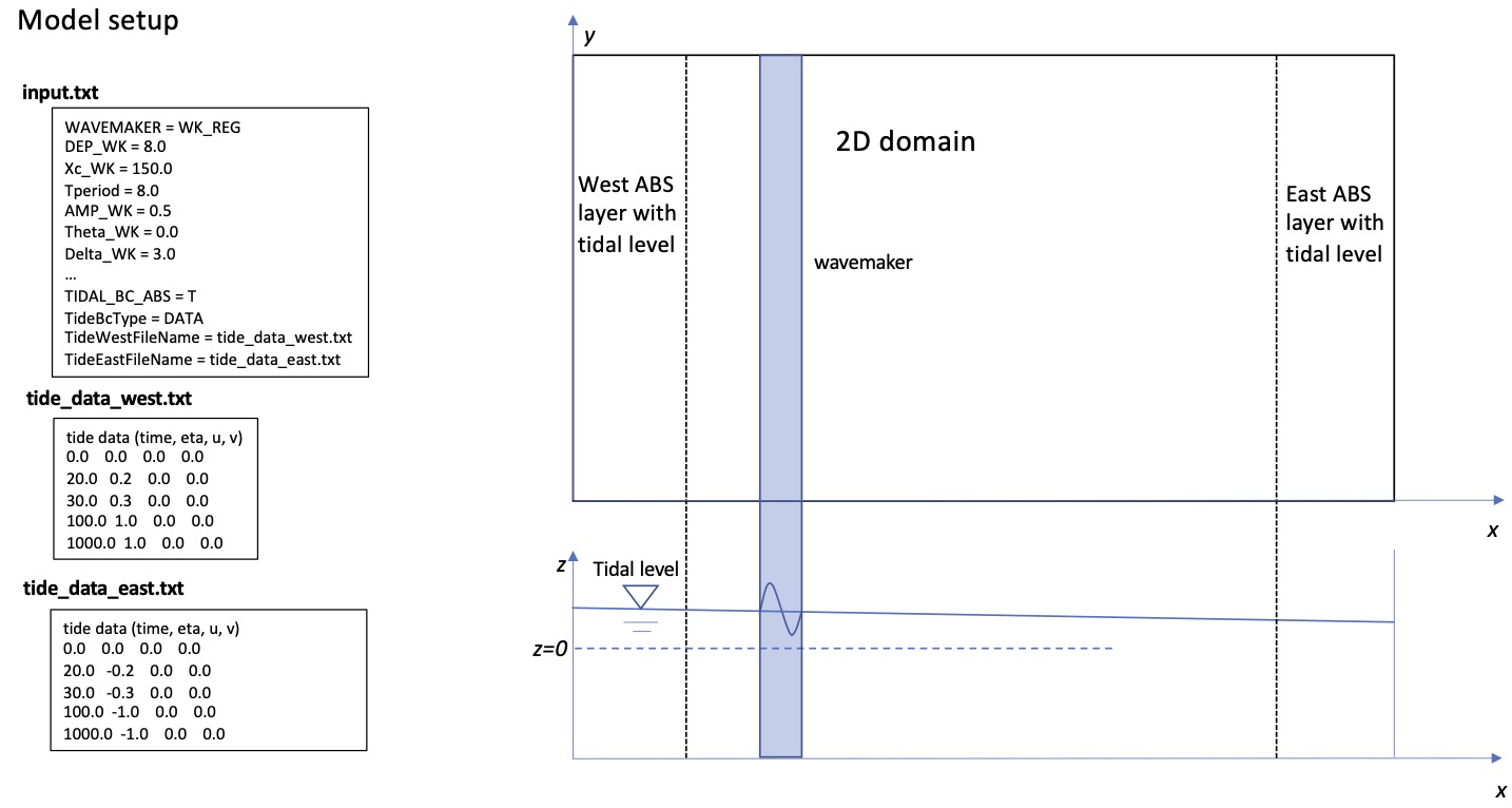
Fig. 2 Layout of tidal absorbing boundary (west and east).

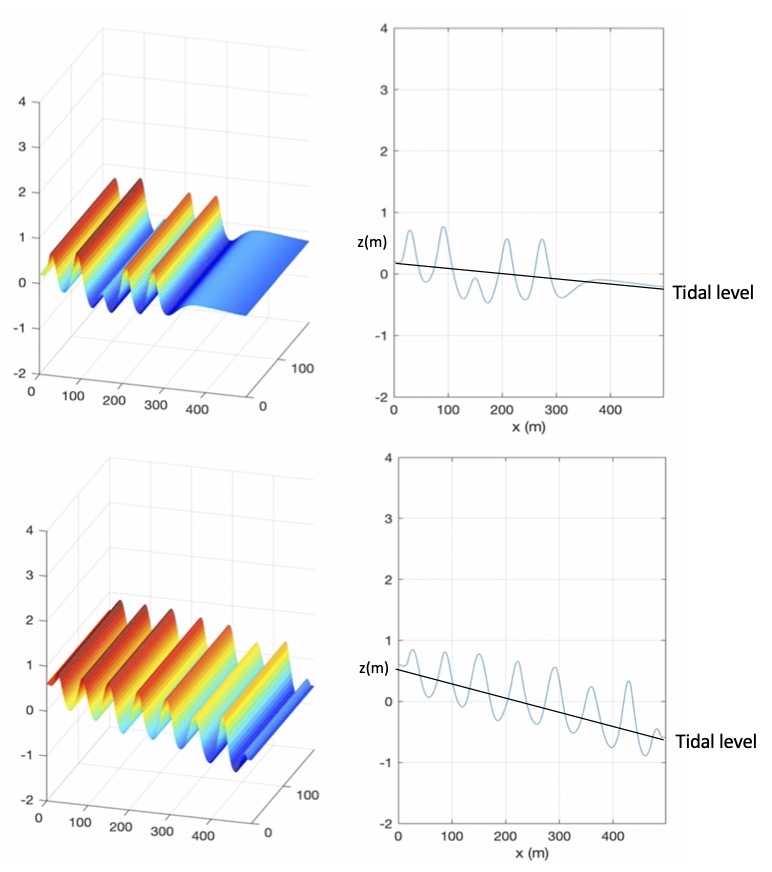
Fig. 3 Case: /simple_cases/tide_abs_2bc_data/. Demonstration of 2D and 1D section views of surface elevation at different times. Black solid lines denote tidal levels.

Combined tidal and absorbing-generating boundary condition

The combined tidal and absorbing-generating boundary condition incorporates the solution of the linear wave theory and tidal elevation and velocity in the sponge layer.

The reference values (\(\eta_{ref}, u_{ref}, v_{ref}\)) are tidal levels and tidal current velocities specified either in input.txt or in a separate tide/surge file. Different from the tidal absorbing boundary condition, the reference values (\(\eta_{ref}, u_{ref}/v_{ref}\)) combine the tidal condition and wave solution, and specified over the entire computational domain. Inside the sponge layer, the differences between the reference values \(( )_{ref}\) and model solution \(( )_i\) are dampened by the sponge. Outside the sponge layer, independent variables are calculated directly from the model because \(C_s\) is 1.0. In this study, the west-side absorbing-generating boundary condition is implemented.

An example is provided In /tide_gen_abs_data/. Figure 4 shows the model setup with a west-side absorbing-generating boundary condition. In input.txt

WAVEMAKER = ABSORBING_GENERATING
WAVE_DATA_TYPE = DATA
WaveCompFile = wave_data.txt
...
TIDAL_BC_GEN_ABS = T
TideBcType = DATA
TideWestFileName = tide_data_west.txt

The format of tidal data is the same as the tidal absorbing boundary condition. The model is set up in a 2D sloping beach domain. Figure 5 shows snapshots of surface elevation at different times.

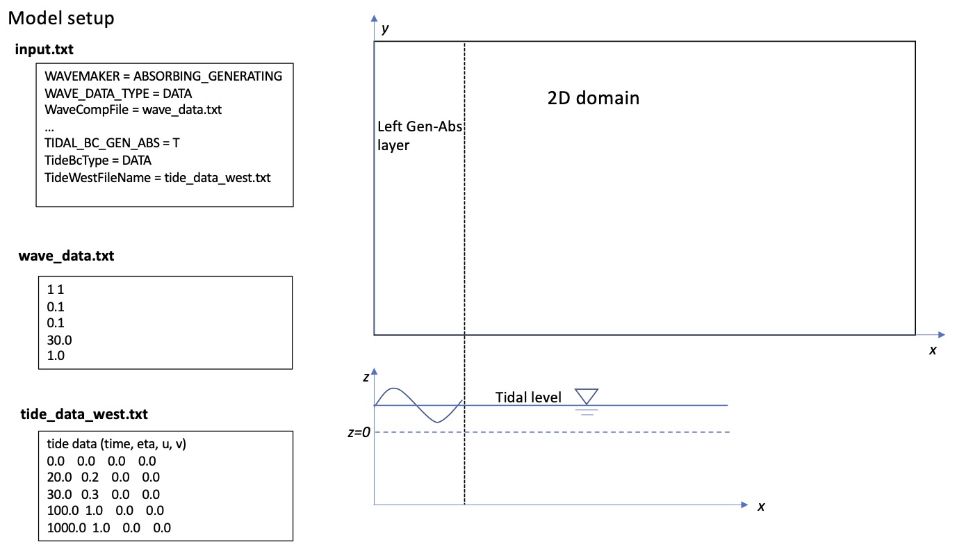
Fig. 4 Layout of generating and absorbing boundary (left only)

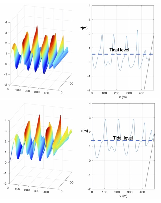
Fig. 5 Case: /simple_cases/tide_gen_abs_data/. Thick dashed lines represent tidal levels. Thin black line denotes the beach slope.

More information

List of parameters for tidal module setup can be found here.

References

Chen, Q., Madsen, P.A., Basco, D.R., 1999. “Current Effects on Nonlinear Interactions of Shallow–Water Waves”. J. of Waterway, Port, Coastal, and Ocean Eng. 125 (4).

Larsen, J. and Dancy, H., 1983. “Open boundaries in short wave simulations – A new approach”. Coastal Eng. 7 (3), 285-297. DOI: 10.1016/0378-3839(83)90022-4.