USERS’ MANUAL
Program outline and flow chart
The code was written using Fortran 90 with the c preprocessor (cpp) statements for separation of the source code. Arrays are dynamically allocated at runtime. Precision is selected using the selected_real_kind Fortran intrinsic function defined in the makefile. The default precision is single.
The present version of NearCoM-TVD includes a number of options including (1) choice of serial or parallel code (2) Cartesian or curvilinear coordinate, (3) samples.
The flow chart is shown in Fig. 4.
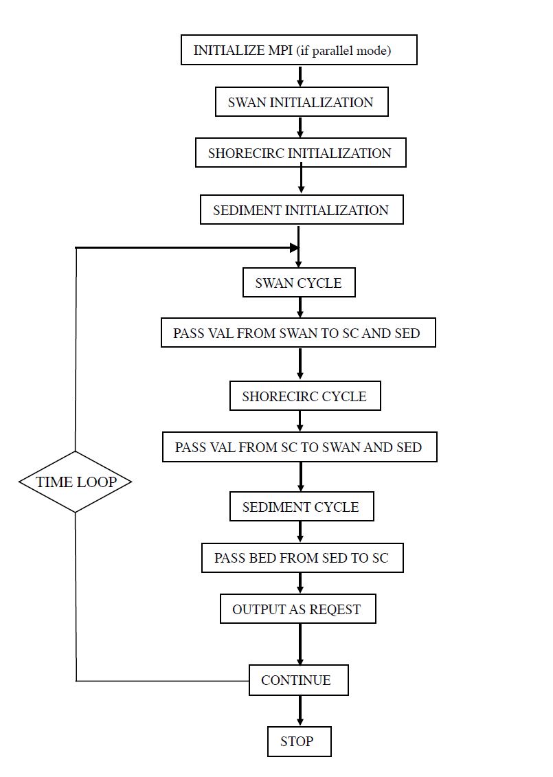
Fig. 4 Flow chart of the main program.
Permanent variables associated with coupling
Depth(): still water depth h at element point
DepthX(): still water depth h at x-interface
DepthY(): still water depth h at y-interface
Eta(): surface elevation, for dry point, Eta() = MinDepth - Depth(), MinDepth is specified in input.txt.
Eta0(): \(\eta\) at previous time level
MASK(): 1 - wet, 0 - dry
MASK_STRUC(): 0 - permanent dry point
U(): depth-averaged u
V(): depth-averaged v
Uc(): contravariant component of depth-averaged velocity in \(\xi_1\) direction
Vc(): contravariant component of depth-averaged velocity in \(\xi_2\) direction
HU(): \((h+\eta)u\) at element
HV(): \((h+\eta)v\) at element
P(): \((h+\eta)U\) at x- interface for Cartesian, and \((h+\eta)Uc\) at \(\xi_1\) -interface curvilinear
Q(): \((h+\eta)V\) at y- interface for Cartesian, and \((h+\eta)Vc\) at \(\xi_2\) -interface curvilinear
Fx(): numerical flux F at x-interface
Fy(): numerical flux F at y-interface
Gx(): numerical flux G at x-interface
Gy(): numerical flux G at y-interface
Ubar(): \(HU\) for Cartesian and \(JHU\) for curvilinear
Vbar(): \(HV\) for Cartesian and \(JHV\) for curvilinear
EtaRxL(): \(\eta\) Left value at x-interface
EtaRxR(): \(\eta\) Right value at x-interface
EtaRyL(): \(\eta\) Left value at y-interface
EtaRyR(): \(\eta\) Right value at y-interface
HxL(): total depth Left value at x-interface
HxR(): total depth Right value at x-interface
HyL(): total depth Left value at y-interface
HyR(): total depth Right value at y-interface
HUxL(): \((h+\eta)u\) Left value at x-interface
HUxR(): \((h+\eta)u\) Right value at x-interface
HVyL(): \((h+\eta)v\) Left value at y-interface
HVyR(): \((h+\eta)v\) Right value at y-interface
PL(): Left P value at x-interface
PR(): Right P value at x-interface
QL(): Left Q value at y-interface
QR(): Right Q value at y-interface
Installation and compilation
NearCoM-TVD is distributed in a compressed fie. To install the programs, first, uncompress the package. Then use
\(>\) tar xvf \(*\).tar
to extract files from the uncompressed package. The exacted files will be distributed in two new directories: /CIRC_SWAN and /work.
To compile the program, go to /CIRC_SWAN and modify Makefile if needed. There are several necessary flags in Makefile needed to specify below.
-DDOUBLE_PRECISION: use double precision, default is single precision.
-DPARALLEL: use parallel mode, default is serial mode.
-DSAMPLES: include all samples, default is no sample included.
- -DCURVILINEAR: curvilinear version, otherwise Cartesian.
\(\bf NOTE:\) setting curvilinear is a must for SWAN and SHORECIRC coupled model.
-DSEDIMENT: include sediment and seabed modules.
-DINTEL: INTEL compiler.
-DRESIDUAL: include tidal residual calculation.
-DSTATIONARY: stationary mode for SHORECIRC
CPP: path to CPP directory.
FC: Fortran compiler.
Then execute
\(>\) make clean
\(>\) make
The executable file ‘nearcom’ will be generated and copied from /CIRC_SWAN to /work/. Note: use ‘make clean’ after any modification of Makefile.
To run the model, go to /work. Modify INPUT if needed and run.
Input
Following are descriptions of parameters in input.txt (\(\bf NOTE:\) all parameter names are capital sensitive).
SWAN INPUT: refer to SWAN manual. Model run time is set in SWAN model. For example,
COMPUTE NONSTAT 20081114.160000 1 MI 20081114.230000
The above setting means model run start from 2008 11 14 16:00 to 2008 11 14 23:00. The model call swan at \(DT_{\mbox{swan}}\) = 1 minute. The loop number for SHORECIRC and SEDIMENT is estimated by \(DT_{\mbox{swan}}\) and the time step of SHORECIRC (time varying).
IMPORTANT SETTING IN SWAN:
in SET, always set CARTESIAN in order to make a grid orientation consistent with SHORECIRC
in SET, always set [inrhog] as 1 to get a true wave energy dissipation.
in COMPUTE, always set NONSTAT mode.
WAVE CURRENT INTERACTION
SWAN_RUN: logical parameter to run SWAN
SHORECIRC_RUN: logical parameter to run SHORECIRC
WC_BOUND_WEST: west bound region (number of grid point) in which wave-current is inactive.
WC_BOUND_EAST : east bound region (number of grid point) in which wave-current is inactive.
WC_BOUND_SOUTH : south bound region (number of grid point) in which wave-current is inactive.
WC_BOUND_NORTH: north bound region (number of grid point) in which wave-current is inactive.
WC_LAG : time delay for wave-current interaction
TITLE:
title for SHORECIRC log file
SPECIFICATION OF MULTI-PROCESSORS
PX: processor numbers in X
- PY: processor numbers in Y
\(\bf NOTE:\) PX and PY must be consistency with number of processors defined in mpirun command, e.g., mpirun -np n (where n = px \(\times\) py).
SPECIFICATION OF WATER DEPTH
DEPTH_TYPE: depth input type.
DEPTH_TYPE=DATA: from a depth file.The program includes several simple bathymetry configurations such asDEPTH_TYPE=FLAT: flat bottom, need DEPTH_FLATDEPTH_TYPE=SLOPE: plane beach along \(x\) direction. It needs three parameters: slope,SLP, slope starting point, Xslp and flat part of depth, DEPTH_FLAT
- DEPTH_FILE: bathymetry file if DEPTH_TYPE=DATA, file dimension should be Mglob x Nglob
with the first point as the south-west corner. The read format in the code is shown below.
DO J=1,Nglob
 READ(1,*)(Depth(I,J),I=1,Mglob)
ENDDO
- DEPTH_FLAT: water depth of flat bottom if DEPTH_TYPE=FLAT or DEPTH_TYPE=SLOPE
(flat part of a plane beach).
SLP: slope if DEPTH_TYPE=SLOPE
Xslp: starting \(x\) (m) of a slope, if DEPTH_TYPE=SLOPE
SPECIFICATION OF RESULT FOLDER
RESULT_FOLDER: result folder name, e.g., RESULT_FOLDER = /Users/fengyanshi/tmp/
SPECIFICATION OF DIMENSION
Mglob: global dimension in \(x\) direction.
- Nglob: global dimension in \(y\) direction.
\(\bf NOTE:\) For parallel runs, Mglob and Nglob can be divided by PX and PY, respectively. MAX(Mglob,Nglob) can be divided by PX \(\times\) PY.
SPECIFICATION OF STATIONARY MODE
- N_ITERATION: the iteration number for stationary mode of SHORECIRC
(set -DSTATIONARY in Makefile).
- WATER_LEVEL_FILE: the file name of water level file containing time and water level, for
stationary mode. The following example shows the format.
water levels for stationary mode5 - number of water level data0.0 0.0 ! Time (s), Level (m)3600.0 0.57200.0 0.866010800.0 1.014400.0 0.86618000.0 0.5
SPECIFICATION OF TIME
PLOT_INTV: output interval in seconds (Note, output time is not exact because adaptive dt is used.)
SCREEN_INTV: time interval (s) of screen print.
PLOT_INTV_STATION: time interval (s) of gauge output
SPECIFICATION OF GRID
DX: grid size(m) in \(x\) direction, for Cartesian mode
DY: grid size(m) in \(y\) direction, for Cartesian mode
X_FILE: name of file to store x for curvilinear mode
- Y_FILE: name of file to store y for curvilinear mode
\(\bf NOTE:\) data format is the same as the depth data shown above.
CORI_CONSTANT: logical parameter for constant Coriolis parameter
LATITUDE: latitude if constant Coriolis parameter is used
- LATITUDE_FILE: name of file to store latitude at every grid point if not constant Coriolis
\(\bf NOTE:\) data format is the same as the depth data shown above.
BOUNDARY CONDITIONS
ETA_CLAMPED: logical parameter for surface elevation clamped condition
V_CLAMPED: logical parameter for velocity clamped condition
FLUX_CLAMPED: logical parameter for flux clamped condition
TIDE_FILE: name of file to store tidal constituents
DATA FORMAT: please refer to mk_tide.f90. The formula of surface elevation at a tidal boundary can be expressed by
where \(a_0\) and \(\phi\) represent amplitude and phase lag, respectively, for a harmonic constituent at location \(\bf x\). \(T\) is tidal period. \(f_c\) and \((V_0+u_0)\) are the lunar node factor and the equilibrium argument, respectively, for a constituent.
The following is an example of M2 + O1.tidal boundary conditions150 — number of days from Jan 1, to simulation date2 — number of constituents1.000 0.000 — \(f_c\) and \((V_0+u_0)\) for M20.980 0.000 — \(f_c\) and \((V_0+u_0)\) for O180 — number of tidal boundary points1 , 1 — (i,j) grid location of tidal boundary12.420 1.200 21.000 — \(T\), amplitude \(a_0\) and phase lag \(\phi\) for M224.000 0.3 30.100 – \(T\), amplitude \(a_0\) and phase lag \(\phi\) for O12 , 1 — (i,j) grid location of tidal boundary12.420 1.200 21.000 — \(T\), amplitude \(a_0\) and phase lag \(\phi\) for M224.000 0.3 30.100 – \(T\), amplitude \(a_0\) and phase lag \(\phi\) for O13 , 1…
FLUX_FILE: name of file to store time series of flux (e.g., unit width river flux)
DATA FORMAT:titleNumber of data, Number of flux pointI, J, River orientationTime, Flux, Angle in Cartesian…where (I,J) represent grid points of river location. River orientation represents the direction which a river flows from in the IMAGE domain (for curvilinear coordinates). Use W,E,S and N for the orientation. For example, ‘W’ represents a river flowing into the domain from the west boundary (in IMAGE domain for curvilinear coordinates).Please refer to mk_river.f90. The following is an example.river flux boundary condition5 2 ! NumTimeData, NumFluxPoint1 38 W ! I, J, River_Orientation0.000 0.200 0.000360000.000 0.200 0.000720000.000 0.200 0.0001080000.000 0.200 0.0001440000.000 0.200 0.0001 39 W ! I, J, River_Orientation0.000 0.200 0.000360000.000 0.200 0.000720000.000 0.200 0.0001080000.000 0.200 0.0001440000.000 0.200 0.000end of file
WIND CONDITION
Spatially uniform wind field is assumed in this version.
WindForce: logical parameter for wind condition, T or F.
WIND_FILE: name of file for a time series of wind speed.
DATA FORMAT: the following is an example of wind data.
wind data100 - number of data0.0 , -10.0 0.0 — time(s), wu, wv (m/s)2000.0, -10.0, 0.08000.0, -10.0, 0.0…
Cdw: wind stress coefficient for the quadratic formula.
SPECIFICATION OF INITIAL CONDITION
INT_UVZ : logical parameter for initial condition, default is FALSE
ETA_FILE: name of file for initial \(\eta\), e.g., ETA_FILE= /Users/fengyanshi/work/input/CVV_H.grd, data format is the same as depth data.
U_FILE: name of file for initial \(u\), e.g.,U_FILE= /Users/fengyanshi/work/input/CVV_U.grd, data format is the same as depth data.
V_FILE: name of file for initial \(v\), e.g., V_FILE= /Users/fengyanshi/work/input/CVV_V.grd, data format is the same as depth data.
SPECIFICATION OF WAVEMAKER
There is no wavemaker implemented in SHORECIRC.
SPECIFICATION OF PERIODIC BOUNDARY CONDITION
(Note: only south-north periodic condition was implemented)
PERIODIC_X: logical parameter for periodic boundary condition in x direction, T - periodic, F - wall boundary condition.
PERIODIC_Y: logical parameter for periodic boundary condition in x direction.
Num_Transit: grid numbers needed to make periodic condition for SWAN. The reason to set this parameter is that SWAN doesn’t have an option for periodic boundary condition. In this implementation, a periodic boundary condition is implemented by making a transition from a left array ( count to Num_Transit from left boundary) to a right array.
SPECIFICATION OF SPONGE LAYER
SPONGE_ON: logical parameter, T - sponge layer, F - no sponge layer.
Sponge_west_width: width (m) of sponge layer at west boundary.
Sponge_east_width: width (m) of sponge layer at east boundary.
Sponge_south_width: width (m) of sponge layer at south boundary.
Sponge_north_width width (m) of sponge layer at north boundary
R_sponge: decay rate in sponge layer. Its values are between 0.85 \(\sim\) 0.95.
A_sponge: maximum damping magnitude. The value is \(\sim\) 5.0.
SPECIFICATION OF OBSTACLES
OBSTACLE_FILE: name of obstacle file. 1 - water point, 0 - permanent dry point. Data dimension is (Mglob \(\times\) Nglob). Data format is the same as the depth data.
SPECIFICATION OF PHYSICS
Cd: quadratic bottom friction coefficient
nu_bkgd : background eddy viscosity parameter.
SPECIFICATION OF NUMERICS
Time_Scheme: stepping option, Runge_Kutta or Predictor_Corrector (not suggested for this version).
HIGH_ORDER: spatial scheme option, FOURTH for the fourth-order, THIRD for the third-order, and SECOND for the second-order (not suggested for Boussinesq modeling).
CONSTRUCTION: construction method, HLL for HLL scheme, otherwise for averaging scheme.
CFL: CFL number, CFL \(\sim\) 0.5.
FroudeCap: cap for Froude number in velocity calculation for efficiency. The value could be 5 \(\sim\) 10.0.
MinDepth: minimum water depth (m) for wetting and drying scheme. Suggestion: MinDepth = 0.001 for lab scale and 0.01 for field scale.
MinDepthFrc: minimum water depth (m) to limit bottom friction value. Suggestion: MinDepthFrc = 0.01 for lab scale and 0.1 for field scale.
SPECIFICATION OF TIDAL RESIDUAL
T_INTV_mean: time-averaging interval for Eulerian mean current and elevation. Note: use -DRESIDUAL in Makefile to make this option active.
SPECIFICATION OF SEDIMENT CALCULATION
Note: set -DSEDIMENT in Makefile to make sediment module active
T_INTV_sed: time interval to call sediment module
Factor_Morpho: morphology factor.
D_50 : \(D_{50}\)
D_90 : \(D_{90}\)
por: sediment porosity
RHO: water density
nu_water: water eddy viscosity
S_sed: specific gravity
SOULSBY: logical parameter for Soulsby (1997) total load formula, T = true, F = false
z0: \(z_0\), bed roughness length.
KOBAYASHI: logical parameter for KOBAYASHI’s formula, T = true, F = false
angle_x_beach: coordinate rotation angle defined in Figure 1.
eB: \(e_B\), suspension efficiency for energy dissipation rate due to wave breaking
ef: \(e_f\), suspension efficiency for energy dissipation rate due to bottom friction
a_k: \(a\), empirical suspended load parameter.
b_k: \(b\), empirical bedload parameter.
TanPhi: \(\tan \phi\), where \(\phi\) is the angle of internal friction of the sediment.
Gm: \(G_m\) for slope function (\(G_m=10\)).
frc: friction coefficient in Kobayashi.
Si_c: a coefficient in calculating \(P_b\).
SPECIFICATION OF OUTPUT VARIABLES
NumberStations: number of station for output. If NumberStations \(> 0\), need input i,j in STATION_FILE
DEPTH_OUT: logical parameter for output depth. T or F.
U: logical parameter for output \(u\). T or F.
V: logical parameter for output \(v\). T or F.
ETA: logical parameter for output \(\eta\). T or F.
HS: logical parameter for output of significant wave height \(H_s\). T or F.
WFC: logical parameter for output of wave force. T or F.
WDIR: logical parameter for output of peak wave direction. T or F.
WBV: logical parameter for output of wave orbital velocity. T or F.
MASK: logical parameter for output wetting-drying MASK. T or F.
SourceX: logical parameter for output source terms in \(x\) direction. T or F.
SourceY: logical parameter for output source terms in \(y\) direction. T or F.
UV3D: logical parameter for output 3D structure. T or F.
Qstk: logical parameter for output Stokes mass flux. T or F.
DepDt: logical parameter for output depth variation rate. T or F.
Qsed: logical parameter for output sediment transport rate. T or F.
Output
The output files are saved in the result directory defined by RESULT_FOLDER in INPUT. For outputs in ASCII, a file name is a combination of variable name and an output series number such eta_0001, eta_0002, …. The format and read/write algorithm are consistent with a depth file. Output for stations is a series of numbered files such as sta_0001, sta_0002 ….