FORMULATIONS

SHORECIRC equations

SHORECIRC is a quasi-3D nearshore circulation model for prediction of wave-induced nearshore circulation. It is a 2D horizontal model which incorporates the effect of the vertical structure of horizontal flows. In Putrevu and Svendsen (1999), the instantaneous horizontal velocity is split as

(1)\[u^{ins}_{\alpha}=u^{\prime}_{\alpha}+u_{w\alpha}+u_{\alpha}+u_{1\alpha}\]

where \(u^{\prime}_{\alpha}, u_{w\alpha}, u_{\alpha}\) and \(u_{1 \alpha}\) are, respectively, the turbulence component, the wave component, the component of depth-averaged and short-wave-averaged velocity, and the vertical variation of the short-wave-averaged velocity. The complete SHORECIRC equations can be expressed in the Cartesian form as in Svendsen et al. (2003) or in the curvilinear form in Shi et al. (2003). In this section, we derive a conservative form of the equations in generalized curvilinear coordinates in order to use the TVD numerical scheme.

SHORECIRC equations in Cartesian coordinates \((x_1, x_2)\) can be expressed as

(2)\[\frac{\partial \eta}{\partial t}+\frac{\partial Hu_\alpha}{\partial x_\alpha} =0\]

(3)\[\frac{\partial H u_\alpha}{\partial t} + \frac{Hu_\alpha u_\beta}{\partial x_\beta} +f_{\alpha}+ g H \frac{\partial \eta}{\partial x_\alpha} + \frac{1}{\rho} \frac{\partial T_{\alpha \beta}}{\partial x_\beta} + \frac{1}{\rho} \frac{\partial S_{\alpha \beta}}{\partial x_\beta} + \frac{\tau^b_\alpha}{\rho} - \frac{\tau^s_\alpha}{\rho} + \mbox{ROT}= 0\]

where \(\eta\) represents the wave-averaged surface elevation, \(H = \eta + h\), in which \(h\) is still water depth. The depth-averaged and wave-averaged velocity \(u_\alpha\) is defined by the ‘Lagrangian’ averaging as

(4)\[u_{\alpha} = \frac{1}{H} \overline{\int_{-h}^\zeta u^{ins}_\alpha}\]

where \(\zeta\) is the instantaneous surface elevation. This split is different from Haas et al. (2003) who used the ‘Eulerian’ concept for their split. For the Lagrangian averaging method, it is assumed that

(5)\[{\int}_{-h}^\eta u_{1\alpha} dz = - Q_{w \alpha}\]

where \(Q_{w \alpha}\) is the short wave flux.

In (3), \(f_\alpha\) represents the Coriolis force which was not considered in the previous SHORECIRC equations (Putrevu and Svendsen, 1999). \(T_{\alpha \beta}, S_{\alpha \beta}, {\tau}^{s}_{\alpha}\) and \({\tau}^{b}_{\alpha}\) are the depth-integrated Reynolds’ stress, the wave-induced radiation stress (Longuet-Higgins and Stewart, 1962, 1964), the surface shear stress and the bottom shear stress, respectively. ROT represents the rest of terms associated with 3D dispersion terms which are not presented here because they do not involve the coordinate transformation conducted below. Interested readers are referred to Putrevu and Svendsen (1999).

A curvilinear coordinate transformation is introduced in the general form

(6)\[xi^1 = \xi^1 (x_1,x_2), \ \ \ \ \xi^2 = \xi^2 (x_1,x_2)\]

where \((\xi^1, \xi^2)\) are the curvilinear coordinates. We use superscript indices, i.e., \(()^\alpha\), to represent the contravariant component and subscript indices for the Cartesian component of a vector. The relation between the Cartesian component \(u_\alpha\) and the contravarient component \(u^\alpha\) can be written, by definition, as

(7)\[u^\alpha = u_\beta L^\alpha_\beta\]

where

(8)\[L^\alpha_\beta = \frac{\partial \xi^\alpha}{\partial x_\beta}\]

Using the chain rule, the derivative of a function \(F\) with respect to \(x_\alpha\) in the Cartesian coordinates can be expressed in the curvilinear coordinates \(\xi^\alpha\) by

(9)\[\frac{\partial F}{\partial x_\alpha} = L^\beta_\alpha \frac{\partial F}{\partial \xi^\beta}\]

Using the metric identity law (Thompson et al., 1985):

(10)\[\frac{\partial}{\partial \xi^\alpha}(J L^\alpha_\beta) \equiv 0\]

(9) can be rewritten in a different form as

(11)\[\frac{\partial F}{\partial x_\alpha} = \frac{1}{J} \frac{\partial F J L^\beta_\alpha}{\partial \xi^\beta}\]

Using (11), the conservative form of SHORECIRC equations in curvilinear coordinates can be derived as

(12)\[frac{\partial \eta}{\partial t} + \frac{1}{J}\frac{\partial J P^\alpha}{\partial \xi^\alpha} = 0\]

(13)\[\begin{split}& \frac{\partial Hu_\alpha}{\partial t} + \frac{1}{J} \frac{\partial }{\partial \xi^\beta} \left[ JP^\beta u_\alpha +\frac{1}{2} g (\eta^2 +2 \eta h) J L^\beta_\alpha \right] +f_\alpha - g \eta \frac{1}{J} \frac{\partial }{\partial \xi^\beta} (h J L^\beta_\alpha) \\ & + \frac{1}{\rho} \frac{1}{J} \frac{\partial }{\partial \xi^\gamma} (S_{\alpha \beta} J L^\gamma_\beta) + \frac{1}{J} \frac{\partial }{\partial \xi^\gamma} (\tau_{\alpha \beta} JHL^\gamma_\beta)+ \frac{\tau^b_\alpha}{\rho} - \frac{\tau^s_\alpha}{\rho} + \mbox{ROT} = 0\end{split}\]

Note that equations (12) and (13) contain both the Cartesian and contravariant variables, which are different from the contravariant-only form in Shi et al., (2003). A difficulty in deriving the conservative form of the momentum equations using contravariant-only variables has be noticed by several authors (e.g., xxx) in shallow water applications. Here, we follow Shi and Sun (1995) who used both Cartesian and contravariant variables in the derivation of the momentum equations.

In (12) and (13), \(P^\alpha = H u^\alpha\), denotes the contravariant component of volume flux, the Coriolis force \(f_\alpha\) uses the Cartesian components, i.e., \((-f H v, fH u)\), \(S_{\alpha \beta}\) represents the Cartesian component of radiation stress. In the present application, the gradient of radiation stresses (the fifth term of (13)) is obtained directly from the wave module SWAN. \(\tau_{\alpha \beta}\) represents the Cartesian component of turbulent shear stress, \(\tau^b_\alpha\) and \(\tau^s_\alpha\) are the Cartesian components of bottom stress and wind stress.

In the derivation of the momentum equations, the surface gradient term is treated following Shi et al. (2011) who reorganized this term in order to make it well-balanced in a MUSCL-TVD scheme for a general order. The expression in curvilinear coordinates can be written as

(14)\[-gHJ\frac{\partial \eta}{\partial x_\alpha} = -\frac{\partial }{\partial \xi^\alpha} \left [\frac{1}{2} g (\eta^2 +2 \eta h) J L^\alpha_\beta \right] + g \eta \frac{\partial }{\partial \xi^\alpha} (h J L^\alpha_\beta)\]

There are several advantages in using equations (12) and (13) versus the contravariant-only form in Shi et al. (2003). First, they are a conservative form which can be implemented using a hybrid numerical scheme. Second, all forcing terms resume to a vector form in Cartesian coordinates in contrast to the contravariant form in Shi et al. (2003). Third, the radiation stress term \(S_{\alpha \beta}\) uses the original form defined in Cartesian coordinates, thus that there is no need to make a transformation for the second-order tensor. The disadvantage is that (13) contains both the Cartesian component \(u_\alpha\) and the contravariant component \(P^\alpha\). However, in terms of the hybrid numerical scheme used in the study, it is convenient to solve both of the two variables using the explicit numerical scheme, rather than the implicit numerical scheme used in Shi et al., (2007).

Wind stress in SHORECIRC was computed using Van Dorn’s (1953) formula:

(15)\[\tau^s_\alpha = f_a \rho_a |{\bf W}| W_{\alpha}\]

where \({\bf W}\) is wind speed at a 10 \(m\) elevation above the water surface, \(f_a\) is the drag coefficient which can be found in Dean and Dalrymple (1991). \(\rho_a\) represents air density. For the bottom stress in SHORECRC, we adopted the formulation for wave-averaged bottom stress for combined currents and waves given by Svendsen and Putrevu (1990) which is written as

(16)\[\tau^b_\alpha = f_{cw} \rho u_0 (\beta_1 u_{b \alpha} +\beta_2 U_{w \alpha})\]

where \(U_{w \alpha}\) is the amplitude of short-wave particle velocity evaluated at the bottom using wave bulk parameters, \(f_{cw}\) is the friction factor, \(u_{b\alpha}\) is the current velocity at the bottom obtained from the theoretical solution of the equation for the vertical variation, \(\beta_1\) and \(\beta_2\) are the weight factors for the current and wave motion given by Svendsen and Putrevu (1990) and evaluated using linear wave theory.

The equation governing the vertical structure of horizontal velocity can be solved analytically using the lowest order of the equation for vertical variation of current:

(17)\[\frac{\partial u_{1\alpha}}{\partial t} -\frac{\partial }{\partial z} \left( \nu_t \frac{\partial u_{1\alpha}}{\partial z}\right) = F_\alpha\]

where \(\nu_t\) is the eddy viscosity coefficient; and \(F_\alpha\) is a general form of the local forcing described as

(18)\[F_\alpha = \frac{1}{\rho h} f_{w\alpha} - f^{lrad}_\alpha + \frac{\tau^b_\alpha}{\rho h} - \frac{\tau^s_\alpha}{\rho h}\]

where \(f_\alpha^{lrad}\) represents the local radiation stress defined by Putrevu and Svendsen (1999). In the offshore domain without wave forcing, (18) reduces to

(19)\[F^\alpha = \frac{\tau^b_\alpha}{\rho h} - \frac{\tau^s_\alpha}{\rho h}\]

The solution of equation (17) can be solved analytically following Putrevu and Svendsen (1999). The bottom current velocity \(u_{b \alpha}\) can be evaluated using \(u_\alpha\) and \(u_{1\alpha}\) at bottom:

(20)\[u_{b \alpha} = u_\alpha + u_{1\alpha} (z=-h)\]

SWAN equations

In this section, we briefly summarize equations used in SWAN. Detailed documentation is referred to SWAN Users’ Manual at http://swanmodel.sourceforge.net/.

The spectral wave model SWAN (Booij et al., 1999, Ris et al., 1999) solves the wave action balance equation. In generalized curvilinear coordinates, the governing equation reads

(21)\[\frac{\partial N}{\partial t} + \frac{1}{J}\frac{\partial (JC_g^\alpha)}{\partial \xi_\alpha} + \frac{\partial (C_{g\sigma}N)}{\partial \sigma} + \frac{\partial (C_{g\theta}N)}{\partial \theta} = \frac{S}{\sigma}\]

where \(\xi_\alpha\) represents curvilinear coordinates defined as the same as in the curvilinear SHORECIRC equations; \(\sigma\) is the relative angular frequency; \(\theta\) is propagation direction of each wave component; \(C_g^\alpha\) represents contravariant component of the energy propagation speed which can be obtained using coordinate transformation:

(22)\[C_g^\alpha = C_{g\beta} L^\alpha_\beta\]

in which \(C_{g_\beta} = (C_{gx}, C_{gy})\) in the rectangular Cartesian coordinates. Equation (21) is written in a tensor-invariant form in order to make it consistent with the circulation equations. The extended numerical form can be found in Booij et al. (1997). \(C_{g\sigma}\) and \(C_{g \theta}\) denote energy propagation speeds in the \(\sigma\) and \(\theta\)-spaces, respectively; \(S\) represents source and sink term in terms of energy density representing the effects of wave generation, dissipation and nonlinear wave-wave interactions; \(N\) is wave action defined by

(23)\[N = E (\xi^\alpha, \sigma,\theta, t) / \sigma\]

in which \(E\) is wave energy density.

Current effects on wave transformation are presented by the following calculations:

1.total group velocity including the current component

(24)\[C_{g\alpha} = \frac{1}{2}\left( 1+ \frac{2kd}{\sinh2kd}\right)\frac{\sigma k_\alpha}{|{\bf k}|^2} + u_{E\alpha}\]

where \(k_\alpha\) or \({\bf k}\) represent wave number, \(d\) is short-wave-averaged water depth, and \(d = h + \eta\). \(u_{E\alpha} = u_\alpha-Q_{w\alpha}/H\) in terms of undertow or Eulerian mean velocity.

2.changes to relative frequency

(25)\[C_\sigma = \frac{\partial \sigma}{\partial d}\left( \frac{\partial d}{\partial t} + {\bf u_E} \cdot \nabla d\right) -C_g \bf{k}\cdot \frac{\partial {\bf u_E}} {\partial {\it s}}\]

3.wave refraction by current included in

(26)\[C_\theta = - \frac{1}{k} \left( \frac{\partial \sigma}{\partial d} \frac{\partial d}{\partial m} +\bf{k}\cdot \frac{\partial {\bf u_E} }{\partial {\it m} } \right)\]

where \(s\) is the space coordinate in direction \(\theta\) and \(m\) is a coordinate normal to \(s\).

Soulsby’s sediment transport formula

The total load transport by waves plus currents derived by Soulsby’s (1997) can be written as

(27)\[q_\alpha = A_s z u_\alpha \left[ \left( u_\alpha^2 + \frac{0.018}{C_d} u_{rms}^2 \right)^{1/2} - u_\alpha^{cr} \right]^{2.4} (1-1.6\tan \beta)\]

where

(28)\[A_{sb} = \frac{0.005 h (d_{50}/d)^{1.2}}{\left[ (s-1)g d_{50}\right]^{1.2}}\]

(29)\[A_{ss} = \frac{0.012 d_{50}D_*^{-0.6}}{\left[ (s-1)g d_{50}\right]^{1.2}}\]

(30)\[A_s = A_{sb} + A_{ss}\]

\(u_{rms}\) is root-mean-square wave orbital velocity; \(C_d\) is drag coefficient due to current alone; \(u_\alpha^{cr}\) represents threshold current velocity given by Van Rijn (1984); \(\beta\) is the slope of bed in streamwise direction; \(s\) is the specific gravity; and

(31)\[D_* = \left[ \frac{g(s-1)}{\nu} \right]^{1/3} d_{50}\]

Kobayashi’s sediment transport formula

Kobayashi et al. (2007) recently proposed sediment transport formulas for the cross-shore and longshore transport rates of suspended sand and bedload on beaches based on laboratory experiment and field data. For suspended sand, the suspended sediment volume \(V_s\) per unit horizontal bottom area was introduced as

(32)\[V_s = P_s \frac{e_B D_r + e_f D_f}{\rho g (s-1) w_f} (1+S_b^2)^{0.5}\]

where \(S_b\) is cross-shore bottom slope; \(e_B\) and \(e_f\) are suspension efficiencies for energy dissipation rates \(D_r\) and \(D_f\) due to wave breaking and bottom friction, respectively. \(w_f\) is the sediment fall velocity; \(P_s\) is the probability of sediment suspension formulated in Kobayashi et al. (2007). The corresponding cross-shore and alongshore suspended sediment transport rates may be expressed as

(33)\[q_{sc} = a \bar{U}_c V_s; \ \ \ \ \ \ q_{sl} = \bar{V}_l V_s\]

where \(a\) is empirical suspended load parameter; \(\bar{U}_c\) is the Eulerian-mean cross-shore current which consists of wave-induced return flow (undertow) and tidal current in the cross-shore direction; \(\bar{V}_c\) is alongshore current which includes wave-induced alongshore current and tidal current in the alongshore direction. Subscriptions \(c\) and \(l\) represent cross-shore and longshore, respectively (hereafter).

In Kobayashi et al., the vector (\(\bar{U}_c, \bar{V}_l\)) is defined specifically in cross-shore/alongshore directions which may not be appropriate for general 2-D applications, especially for complex coastal geometry. Here, we define \(\vec{\bar{V}} = (\bar{U},\bar{V})\) as the Eulerian-mean current vector in general Cartesian coordinates which may not be restricted to the cross-shore/alongshore orientation. Thus formula (33) can be written in a general form using coordinate rotation as

(34)\[q_{sx} =( a \bar{U} \cos^2 \alpha + a \bar{V} \sin \alpha \cos \alpha + \bar{U} \sin^2 \alpha -\bar{V}\sin \alpha \cos \alpha) V_s\]

(35)\[q_{sy} = (a \bar{V} \sin^2 \alpha + a \bar{U} \sin \alpha \cos \alpha + \bar{V} \cos^2 \alpha -\bar{U}\sin \alpha \cos \alpha) V_s\]

in which \(\alpha\) is an angle between \(x-\) axis and beach-normal direction as shown in Fig. 1.

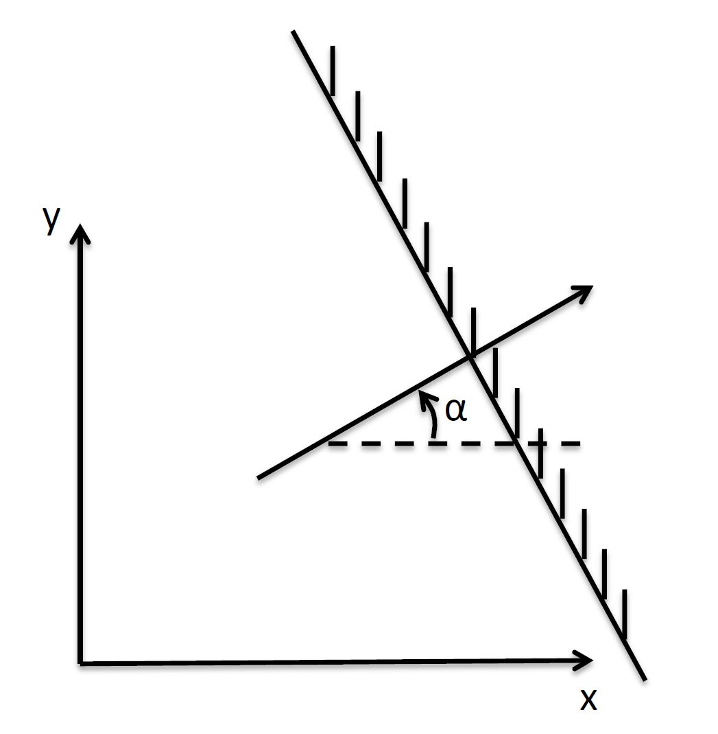
Fig. 1 Definition of an angle between \(x-\) axis and beach-normal direction.

The bedload transport rates can be expressed as

(36)\[q_{bc} = \frac{b P_b}{g (s-1)} \sigma^3_T (1+ U_* V_*^2 +2 F_m \sin \theta) G_s\]

(37)\[q_{bl} = \frac{b P_b}{g (s-1)} \sigma^3_T \left[ V_* (1+U^2_* + V^2_*) -2 r_m \sin \theta \right ]\]

where \(b\) is empirical bedload parameter; \(\sigma_T\) is standard deviation of the oscillatory depth-averaged velocity with zero mean; \((U_*, V_*) = (\bar{U}_c/\sigma_T, \bar{V}_l/\sigma_T)\); \(\theta\) is wave angle; and

(38)\[r_m = -(U_*\cos \theta + V_* \sin \theta)\]

(39)\[F_m = V_* \cos \theta - U_* \sin \theta\]

\(G_s\) is the bottom slope function expressed by

(40)\[\begin{split}\begin{array}{l l l} G_s = \tan \phi /(\tan \phi + S_b) & \mbox{for} & -\tan \phi < S_b < 0 \\ G_s = (\tan \phi -2 S_b) /(\tan \phi -S_b) & \mbox{for} & 0 < S_b < \tan \phi \end{array}\end{split}\]

in which \(\phi\) is the angle of internal friction of the sediment and \(\tan \phi \simeq 0.63\) for sand.

In a general Cartesian system, (\(q_{bc}, q_{bl}\)) are converted to (\(q_{bx}, q_{bl}\)) using

(41)\[q_{bx} = q_{bc} \cos \alpha - q_{bl} \sin \alpha, \ \ \ \ \ \ q_{by} = q_{bc} \sin \alpha + q_{bl} \cos \alpha\]

Seabed evolution equation

The sea bed evolution equation can be described using sediment transport flux in generalized curvilinear coordinates:

(42)\[(1-p) \frac{\partial h}{\partial t} + \frac{1}{J} \frac{\partial J f_{mor} q_\beta L^\alpha_\beta}{\partial \xi^\alpha} = 0\]

where \(p\) is the bed porosity, \(f_{mor}\) represents a morphology factor. (42) is solved using the same TVD scheme as in SHORECIRC.